Lab 5.3: More aggregations

Objective:

In this lab, you will manipulate more advanced aggregation.

Using the blogs_fixed2 index, write a query that searches for elasticsearch siem in the content field. Use this scope of documents to get the top three blogs of each one of the top five categories. For better visibility, filter the _source to include only the title.

Solution

GET blogs_fixed2/_search
{
  "size": 0, 
  "query": {
    "match": {
      "content": "elasticsearch siem"
    }
  },
  "aggs": {
    "top5_categories": {
      "terms": {
        "field": "category_title.title",
        "size": 5
      },
      "aggs": {
        "top3_blogs": {
          "top_hits": {
            "size": 3,
            "_source": ["title"]
          }
        }
      }
    }
  }
}

In the previous lab, you found the top 3 URLs for each of the top 5 os.

GET web_traffic/_search
{
  "size": 0,
  "aggs": {
    "top_OS": {
      "terms": {
        "field": "user_agent.os.name.keyword",
        "size": 5
      },
      "aggs": {
        "top_urls": {
          "terms": {
            "field": "url.original",
            "size": 3
          }
        }
      }
    }
  }
}

Change the terms aggregation of the top 3 URLs to a significant_terms aggregation and compare the results of the two different queries. Notice how the URLs have changed to be less generic and more specific topics

Solution

GET web_traffic/_search
{
  "size": 0,
  "aggs": {
    "top_OS": {
      "terms": {
        "field": "user_agent.os.name.keyword",
        "size": 5
      },
      "aggs": {
        "top_urls": {
          "significant_terms": {
            "field": "url.original",
            "size": 3
          }
        }
      }
    }
  }
}

What is the hourly sum of bytes_sent?

Solution

GET web_traffic/_search
{
  "size": 0,
  "aggs": {
    "logs_by_hour": {
      "date_histogram": {
        "field": "@timestamp",
        "calendar_interval": "hour"
      },
      "aggs": {
        "sum_bytes": {
          "sum": {
            "field": "bytes_sent"
          }
        }
      }
    }
  }
}

Update the previous query to compute the moving average of the hourly sum. Use a window of 5 hours.

Solution

GET web_traffic/_search
{
  "size": 0,
  "aggs": {
    "logs_by_hour": {
      "date_histogram": {
        "field": "@timestamp",
        "calendar_interval": "hour"
      },
      "aggs": {
        "sum_bytes": {
          "sum": {
            "field": "bytes_sent"
          }
        },
        "the_movfn": {
          "moving_fn": {
            "buckets_path": "sum_bytes",
            "window": 5,
            "script": "MovingFunctions.unweightedAvg(values)"
          }
        }
      }
    }
  }
}

Optional: It is difficult to see the difference using only Console. Let's create a visualization to see the difference in Kibana:
- Open the main menu and click Visualize Library.
- Create a new Lens visualization.
- Select the web_traffic data view and see the correct time range (from April 1 to April 30, 2021.)
- Drag and drop the @timestamp field into the Horizontal axis and customize the time interval to be 1 hour.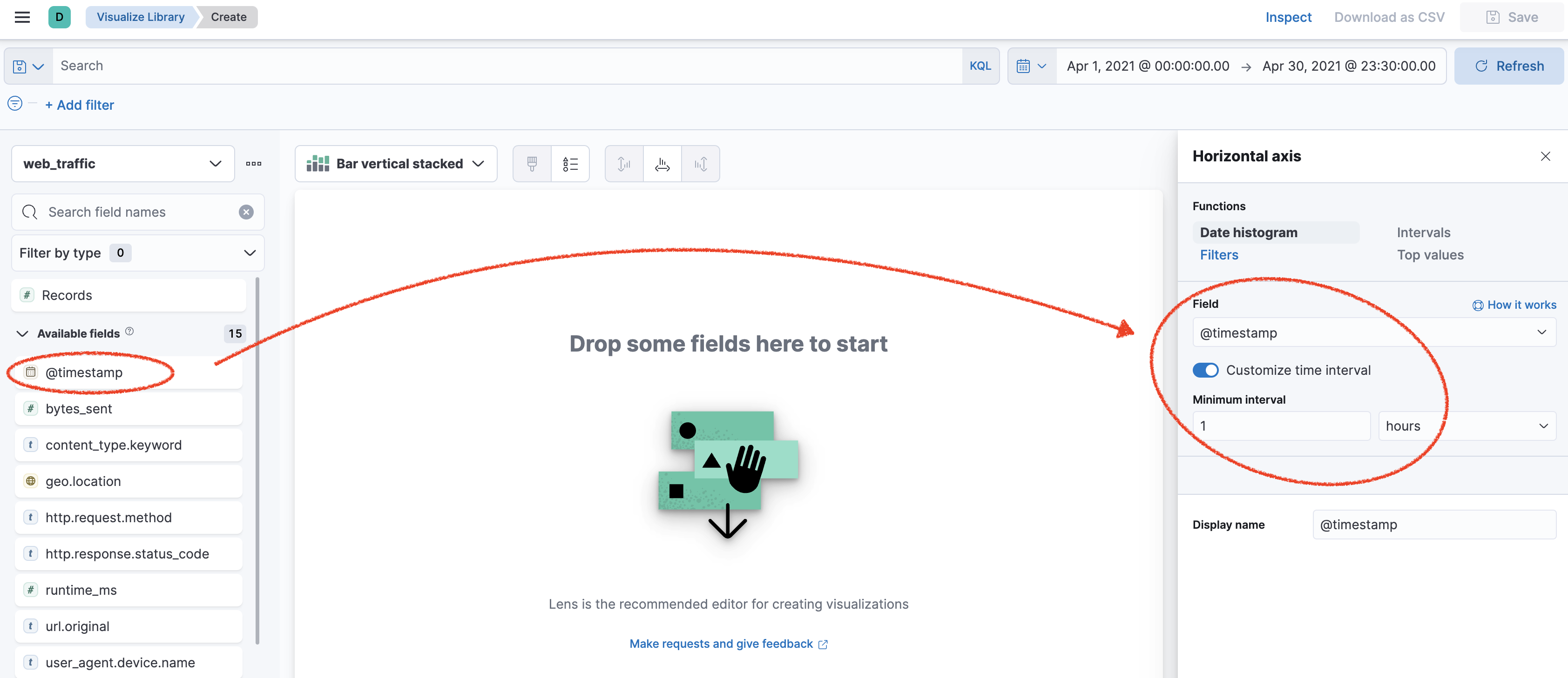
- Drag and drop the bytes_sent field into the Vertical axis and select the sum.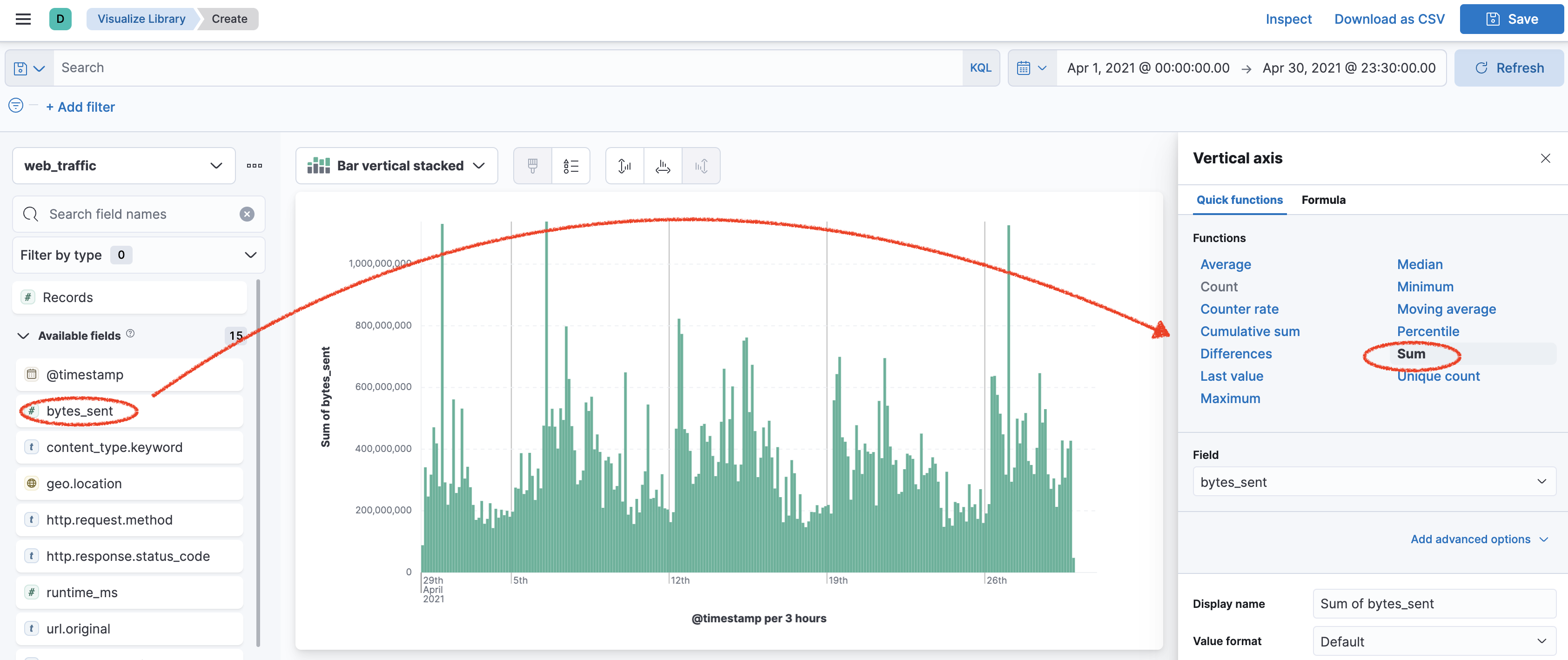
- Next, add a new layer to your visualization.
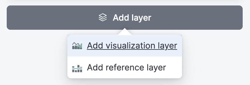
- Select the line visualization.
- Drag and drop the @timestamp field into the Horizontal axis and customize the time interval to be 1 hour.
- Drag and drop the bytes_sent field into the Vertical axis and, this time, select the moving average for the sum of bytes_send.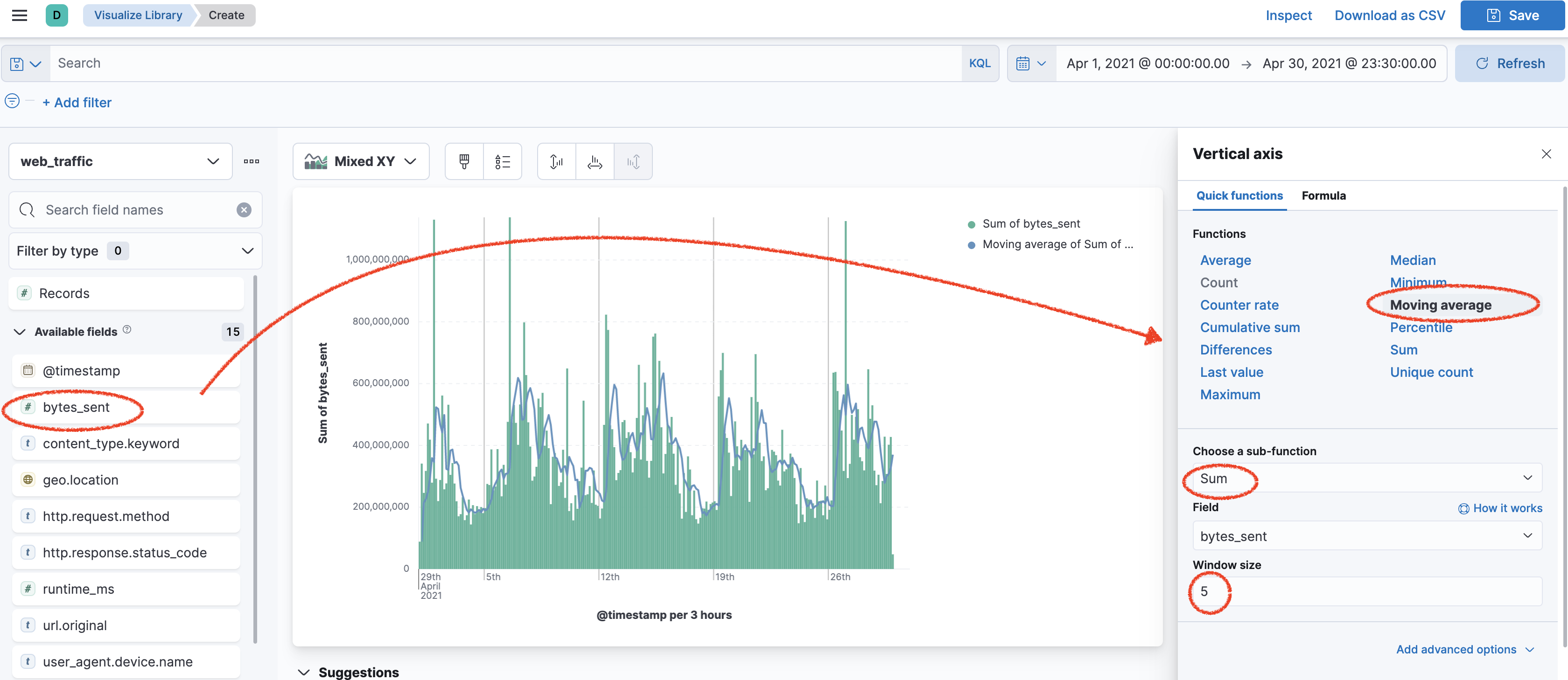

Summary:

You used more advanced aggregations such as top_hits and significant_terms. You computed the moving average using a pipeline aggregation.